基本信息

• authors: Wei Liu, Dragomir Anguelov, Dumitru Erhan, Christian Szegedy, Scott Reed, Cheng-Yang Fu, Alexander C. Berg
• tags: #Object-Detection, #One-Stage
• date: 2016
• note-Date: 2021-10-30
• note: 这篇论文已经比较早了，是2016年发表在ECCV上的一篇论文，从现在的目标检测算法发展的速度来说，已经有一些“久远”了，但是这篇论文依然有很高的引用量，是one-stage中一篇非常经典的论文，主要了解本篇论文主要贡献，学习其模型结构即可。后面的实验部分就直接略过了。

文章内容

Abstract

We present a method for detecting objects in images using a single deep neural network. Our approach, named SSD, discretizes the output space of bounding boxes into a set of default boxes over different aspect ratios and scales per feature map location. At prediction time, the network generates scores for the presence of each object category in each default box and produces adjustments to the box to better match the object shape.

本篇论文主要提出了一个单步的神经网络来进行图像的目标检测任务，这个模型的名字叫做SSD，它可以将边界框的输出空间离散或者叫做映射为一组default box，这些default box覆盖在不同尺寸，不同比例的特征图上。在进行目标检测预测的时候，SSD会对每一个default box上的每一个目标类别生成概率分数，并且会调整这些bounding box去更好的适应不同的目标形状或者尺寸。

the network combines pre-dictions from multiple feature maps with different resolutions to naturally handle objects of various sizes.

这个网络结合了多个来自不同分辨率特征层的预测值来很自然的检测不同大小的目标，大尺寸的特征层拥有更多细节，所以它会尽可能去检测小目标，而小尺寸的特征层抽象程度更高，就更有可能会检测一些大目标。

SSD is simple relative to methods that require object proposals because it completely eliminates proposal generation and subsequent pixel or feature resampling stages and encapsulates all computation in a single network.

SSD相对于需要proposals的方法相对来说简单的，因为SSD完全消除了proposals的生成部分和随后的特征重采样部分并且将所有的对类别的概率预测值和bounding box的回归值预测都封装到了一个网络里。（这里应该是相对于Faster R-CNN来说的）

它的效果也是很好的，在VOC2007上获得了74.3%的mAP，并且一秒可以检测59张图片，速度相比于Faster R-CNN来说快了不知道多少倍。

Introduction

While accurate, these approaches have been too computationally intensive for em-bedded systems and, even with high-end hardware, too slow for real-time applications.

There have been many attempts to build faster detectors by attacking each stage of the detection pipeline, but so far, significantly increased speed comes only at the cost of significantly decreased detection accuracy.

在引言部分，作者首先主要提出在SSD之前所有的目标检测任务都是对Faster R-CNN的改进，虽然Faster R-CNN准确率比较高，但是计算量太大， 在一些高端设备商预测时间都很长，更不要说在嵌入式设备上了，很多人尝试在Faster R-CNN的不同阶段进行改进来提高速度，比如说改进RPN部分，但是大多数速度的提高都是以精度下降为代价的。

This paper presents the first deep network based object detector that does not re-sample pixels or features for bounding box hypothesesandand is as accurate as ap-proaches that do.

The fundamental improvement in speed comes from eliminating bounding box proposals and the subsequent pixel or feature resampling stage.

这篇论文提出了首个基于深度网络的目标检测模型，它不需要对像素进行重采样或者假设bounding box的特征（这里可能的意思就是不需要利用anchor或者proposal吧），模型的实验结果可以显著的提升高精度目标检测速度。模型速度的提升的原因就是完全消除了bounding box proposals和后续的对像素的重采样阶段。

Our improvements include using a small convolutional filter to predict object categories and offsets in bounding box locations, using separate predictors (filters) for different aspect ratio detections, and applying these filters to multiple feature maps from the later stages of a network in order to perform detection at multiple scales.

With these modifications—especially using multiple layers for prediction at different scales—we can achieve high-accuracy using relatively low resolution input, further increasing de-tection speed.

这篇论文的改进主要是：1. 使用了一个小的卷积滤波器去预测目标类别和bounding box位置的偏移，这里需要注意和Faster R-CNN区别，Faster R-CNN在预测bounding box时是对每一个proposal的每一个类别都进行了一组回归值的预测， 而SSD是对每一个default box只进行了一组预测。2. SSD会分别使用不同的预测器进行不同的长宽比检测，并且会将这组预测器应用于网络后期阶段的每一个特征层上，方便在多个尺度上进行检测。

We summarize our contributions as follows: - We introduce SSD, a single-shot detector for multiple categories that is faster than the previous state-of-the-art for single shot detectors (YOLO), and significantly more accurate, in fact as accurate as slower techniques that perform explicit region proposals and pooling (including Faster R-CNN). - The core of SSD is predicting category scores and box offsets for a fixed set of default bounding boxes using small convolutional filters applied to feature maps. - To achieve high detection accuracy we produce predictions of different scales from feature maps of different scales, and explicitly separate predictions by aspect ratio. - These design features lead to simple end-to-end training and high accuracy, even on low resolution input images, further improving the speed vs accuracy trade-off. - Experiments include timing and accuracy analysis on models with varying input size evaluated on PASCAL VOC, COCO, and ILSVRC and are compared to a range of recent state-of-the-art approaches.

这篇论文的主要贡献：

1. 提出一种用于多个类别的单步检测框架SSD，比之前最优的单步检测框架YOLO要更快，并且更准确，它的准确率甚至比使用region proposal和RoI pooling的更慢的技术（包括Faster R-CNN）要更高。
2. SSD的核心是使用应用于特征层的小的卷积滤波器来预测类别分数和基于default bounding boxes的偏移值。
3. 从不同尺度的特征图中生成不同尺度的预测，并且根据不同的宽高比进行不同的预测。
4. 这些设计特性导致简单的端到端训练和高精度，在一些低分辨率的图片上，也能进一步提高准确性。
5. 和其他的一些模型做了对照实验，表明SSD的有效性。

SSD

Model

网络模型框架

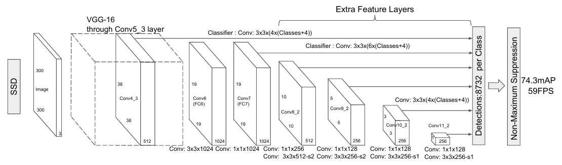
Base network Our experiments are all based on VGG16 [15], which is pre-trained on the ILSVRC CLS-LOC dataset [16]. Similar to DeepLab-LargeFOV [17], we convert fc6 and fc7 to convolutional layers, subsample parameters from fc6 and fc7, change pool5 from 2×2−s2 to 3×3−s1, and use theà trousalgorithm [18] to fill the ”holes”. We remove all the dropout layers and the fc8 layer. We fine-tune the resulting model using SGD with initial learning rate10−3, 0.9 momentum, 0.0005 weight decay, and batch size 32. The learning rate decay policy is slightly different for each dataset, and we will describe details later.

首先，由上图可知，SSD输入的大小是固定的，为300×300大小，也就是说在送入模型之前就要先做一个预处理。然后再送入到这个VGG-16的backbone中进行特征的提取。但是应该注意的是这里用到的VGG-16模型不是用到了所有的层，有几层是修改过的，首先是第五个全连接层之后的pool，原先是一个核大小2×2步长为2，这个操作会使通过conv5出来的特征图缩减为原来的一半，但是将核大小改为3×3步长改为1之后整体的特征图大小是不发生变化的，也就是说通过pool4之后的19×19的特征图经过conv5以及pool5之后大小并没有发生变化，再一个就是将原来VGG-16的两个全连接层（fc6，fc7）修改成了两个卷积层（conv6，conv7），后面又增加了几个卷积层来输出不同大小的特征图，以方便后续在不同的特征图上进行预测。那么那多个特征层是从那些地方得到的呢？首先第一个特征层就是原先VGG-16的conv4得到的特征图特征图大小为38×38×512，第二个特征层是通过Conv7得到的大小为19×19×1024，而第三、四、五、六个特征层都是通过额外添加的卷积层得到的，并且需要注意的是每一个特征图都是通过两个卷积层得到的，其中一个是一个1×1的卷积，另一个是一个3×3的卷积，注意经过3×3卷积的特征图时，当步长为2时padding为1，步长为1时padding为0。

模型架构设计原因

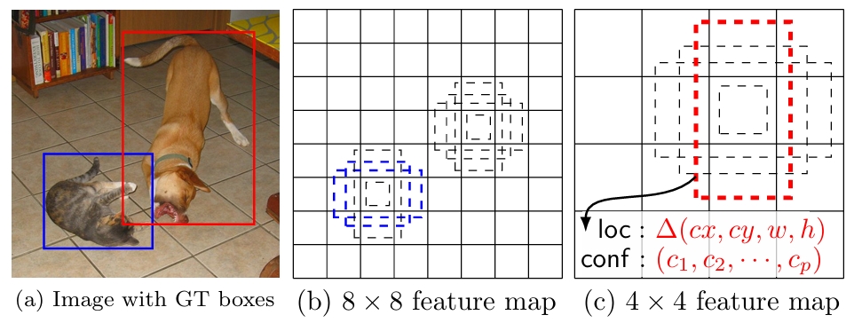
1. SSD only needs an input image and ground truth boxes for each object during training. In a convolutional fashion, we evaluate a small set (e.g. 4) of default boxes of different aspect ratios at each location in several feature maps with different scales (e.g.8×8and4×4in (b) and (c)). For each default box, we predict both the shape offsets and the confidences for all object categories ((c1, c2,· · ·, cp)). At training time, we first match these default boxes to the ground truth boxes. For example, we have matched two default boxes with the cat and one with the dog, which are treated as positives and the rest as negatives. The model loss is a weighted sum between localization loss (e.g. Smooth L1 [6]) and confidence loss (e.g. Softmax).

在Faster R-CNN中无法兼顾小目标的检测，因为整个预测过程都是在一个特征图上进行的，一些细节目标难以考虑到，并且Faster R-CNN两阶段模型每一个阶段都需要在anchor上对类别和bbox回归值进行预测（RPN基于anchor预测一个回归值和前景概率，而后面的FastRCNNPredictor部分则是基于proposal预测回归值和类别概率值，要计算两次损失，而SSD在不同的特征层上定义DefaultBox，直接在这些DefaultBox上进行类别预测和回归值预测，并且每一个特征图上的特征点只预测一个Default Box回归值就可以，而不需要像FasterRCNN一样，在给每一个proposal预测回归时有多少类就要预测多个回归值。只计算一次损失就可以了。并且六个预测特征层预测不同大小的目标，大特征图抽象程度比较低可以用来检测小目标，而特征图越小，抽象程度就越高，就越容易检测大目标。

Choosing scales and aspect ratios for default boxes

Feature maps from different levels within a network are known to have different (empirical) receptive field sizes [13]. Fortunately, within the SSD framework, the de-fault boxes do not necessary need to correspond to the actual receptive fields of each layer. We design the tiling of default boxes so that specific feature maps learn to be responsive to particular scales of the objects. Suppose we want to usemfeature maps for prediction. The scale of the default boxes for each feature map is computed as:

上述文本中描述了SSD框架设计了一种特定的Default Box的tiling，以便特定的特征图能够对特定的屋顶比例做出响应。并且给出了一个Default的计算公式。文章的后一段还详细描述了这个公式的含义。但是在SSD官方实现的代码中，并没有直接使用这一套公式，而是直接给出了每一个特征层的scale和aspect的比例。

原论文还提出来一点：

For the aspect ratio of 1, we also add a default box whose scale is , resulting in 6 default boxes per feature map location.

这里也就是说对于aspect ratio为1的情况，增加了一种scale就是，这里的s_k是第k个scale值，而s_k + 1是第k+1个scale值。

关于scale和aspect ratio的信息原文中还提到：

We use conv43, conv7 (fc7), conv8_2, conv9_2, conv10_2, and conv11_2 to predict both location and confidences. We set default box with scale 0.1 on conv4_3. We initialize the parameters for all the newly added convolutional layers with the ”xavier” method. For conv4_3,conv10_2 and conv11_2, we only associate 4 default boxes at each feature map location omitting aspect ratios of 1/3 and 3. For all other layers, we put 6 default boxes as described in Sec.

上述描述了conv4的第三层和conv10的第三层还有conv11的第2层都有4个Default Box，因为scale为1的Default Box有两个，再加上1:2和2:1的两个Default Box一共就四个Default Box，而剩余的特征层则有六个Default Box因为要加上两个1:3和3:1的Default Box。而在源码中，一共提供了6个scale，他们按照卷积层的顺序分别是[21,45,99,153,207,261,315]，拿conv4_2来说，它应该有四个比例，分别是[1:1, 1:2, 2:1]而1:1有两种情况，所以最后的比例是这样的[21:21, 21:42, 21:10.5, ]，后面乘以的45就是conv7的scale，这样以此类推就可以得到后面几种尺度的Default Box的大小，只不过他们的个数是不一样的。

通过以上的图就能得出一共有8732个Default Box。

Predictor的实现

SSD是如何来进行预测的？

For a feature layer of size m×n with p channels, the basic element for predicting parameters of a potential detection is a 3×3×p small kernel that produces either a score for a category, or a shape offset relative to the default box coordinates.

这里说明了对于m×n且通道为p的一个特征层，直接使用一个3×3×p的小卷积核来对类别分数和相对于Default Box的偏移量。

那每一个特征图会有多少个输出呢？

Specifically, for each box out of k at a given location, we compute c class scores and the 4 offsets relative to the original default box shape. This results in a total of (c + 4) k filters that are applied around each location in the feature map, yielding (c + 4)kmn outputs for a m×n feature map.

对于特征图上的每一个特征点会有k个Default Box，一共有c个类别，所以对每一个Default Box要输出c个类别预测值，对于一个特征点就要预测kc个类别值，对于每个Default Box的回归值，要预测两个坐标也就是4个值，但是要注意的是每一个default Box只需要预测4个回归值就可以了，不用像Faster R-CNN那样，需要每一个proposal对每一个类别预测4个回归值，也就是每一个特征点上会有4k个预测回归值，最后对于一个m×n大小的特征图来说，每个特征点需要预测(c + 4)k个值，整张特征图就要预测(c + 4)kmn个值。

Trarning

正样本选取

We begin by matching each ground truth box to the default box with the best jaccard overlap (as in MultiBox [7]). Unlike MultiBox, we then match default boxes to any ground truth with jaccard overlap higher than a threshold (0.5).

为每一个GTBox匹配IoU值最大的Default Box作为正样本，除此之外，当一个Default Box和GTBox的IoU大于0.5时，这个Default Box也算是正样本。

负样本选择

After the matching step, most of the default boxes are negatives, especially when the number of possible default boxes is large. This introduces a significant imbalance between the positive and negative training examples. Instead of using all the negative examples, we sort them using the highest confidence loss for each default box and pick the top ones so that the ratio between the negatives and positives is at most 3:1. We found that this leads to faster optimization and a more stable training

在正样本匹配完成后，剩下的样本都可以当做负样本，但是当Default Box数量特别多的时候，就会导致正样本和负样本的差距特别大，这就导致了正样本和负样本分布不平衡的问题，所以在训练的时候并不使用所有的负样本进行训练，而只是使用其中的一部分，首先将所有的正样本之外的样本按照一个最高置信度损失进行排序，这个置信度损失越大就表明这个样本就越可能被预测成为一个正样本，而它本身不是正样本，这就表明它和负样本这个分布差距很大，所以就将这类样本设置成为负样本，将排序后的前n个样本作为负样本进行训练，这里的n要和正样本成1:3的关系。

Loss

最后来关注一下损失的部分，SSD的损失和Faster RCNN的损失是类似的，是由类别损失和定位损失组成。

其中N为正样本个数，α为1。(L_conf(x, c)就是类别损失，而L_loc(x, l, g)则是回归损失。

对于类别损失，原文中也直接给出了一个公式，这个公式包含两部分的类别损失，一部分是正样本的类别损失，一部分是负样本的类别损失。

其中这一部分就是正样本的类别损失，而∑_{i ∈ Neg}log (ĉ_i⁰)则是负样本的类别损失。ĉ_i^p为预测的第i个default box对应的GTBox(类别为P)的类别概率，而x_ij^p为第一个default box匹配到的第j个GTBox(类别是P)。

对于定位损失或者说回归损失，只是针对于正样本，因为负样本是不用计算回归值的，所以SSD的定位损失和Faster RCNN是非常像的，就是要计算四个预测回归值和四个GTBox的真实值之间的损失，四个值分别是default box的中心坐标和default box的长和宽。

其中。
ĝ_j^cx = (g_j^cx−d_i^cx)/d_i^w  ĝ_j^cy = (g_j^cy−d_i^cy)/d_i^h
上面的公式就是计算Default Box预测框的中心点和GTBox的中心点之间的差异。

上面的公式是计算Default Box预测框的宽高河GTBox宽高之间的损失。l_i^m为预测对应第i个正样本的回归参数，而ĝ_j^m为正样本i匹配的第j个GTBox的回归参数。

最后把这个四个损失值相加得到整个定位损失值。